Massive new hawk migration spot
By Justin on April 2, 2020
While most Broad-winged Hawks are but a few weeks away from Missouri, the first sightings this year have been trickling in this week as spring migration is off to an early start.
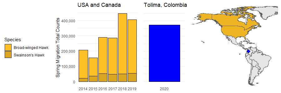
Meanwhile in Colombia, my friend Diego Solarte and his team just concluded counting 373,621 raptors, mostly Broad-winged and Swainson’s Hawks, over one month at a new field station near Ibagué, in the department of Tolima. In the first week they counted 34,108, in the second a whopping 214,582, in the third week 39,587 and finally 58,344 raptors in the last week. Pretty nice! So given that I was working with some eBird data on North American birds at the time, I decided to compare Diego’s counts from Tolima to all Broad-winged and Swainson’s Hawk counts in North America during spring migration, just to put it into perspective.
What I found was that this new site gets close to the total count of raptors that get entered into eBird* in all of North America in the spring! Check at the yearly totals below.
His team has recently started a new raptor counting station in a critical migratory corridor of the central Andes, where many migratory raptors are threatened by illegal hunting. Despite the global COVID-19 outbreak, they have now concluded one month of fieldwork. While the station is up and running, they have yet to reach their campaign funding goal.
If you can, please consider donating to their GoFundMe campaign at the following link: https://www.gofundme.com/f/xrzme-conservation-of-migratory-raptors-in-colombia?utm_source=customer&utm_medium=copy_link-tip&utm_campaign=p_cp+share-sheet
This project offers highly effective “bang-for-your-conservation-buck”: it is a small grassroots organization led by dedicated local birders and biologists, and a few dollars go a long way - especially now due to the recent spike in exchange rate.

And for a glimpse of what they’ve been seeing, check out one incredible checklist from the other week (https://ebird.org/checklist/S66130019).
While this peek into the data was done out of curiosity alone, I am really looking forward to see their real analyses and reports.
*There are a lot of reasons why simple summary statistics like on this plot don’t capture the exact number of hawks in the USA and Canada during spring migration. For example, not all hawk monitoring places submit all their data to eBird. Next, eBird data comes from birders, so if two birders who are out by themselves see the same kettle of hawks, but from different places or at different times of day, those data would be entered in eBird twice. There are lots of tricky modelling techniques that take the peculiarities of eBird data into account, and I am not attempting to replicate any of these. Also, eBird is growing every year, with more and more people reporting, so that is likely why the last five years show increasing numbers in North America.
Reference:
eBird Basic Dataset. Version: EBD_relOct-2019. Cornell Lab of Ornithology, Ithaca, New York. 2019.
Below is my R code for the plot (this works only if you have the eBird Basic Dataset downloaded).
library(auk)
library(tidyverse)
library(lubridate)
library(rworldmap)
library(gridExtra)
library(rnaturalearth)
library(rnaturalearthdata)
library(sf)

bwha<-read_ebd("E:/EBD/data/ebd_brwhaw_relOct2019.txt")
bwha$observation_count<-as.numeric(bwha$observation_count)
bwha<-bwha %>% filter(country_code %in% c("US", "CA") & is.na(observation_count)==F)
bwha$observation_date<-parse_date_time(bwha$observation_date, orders = c("Ymd"))
bwha$month<-month(bwha$observation_date)
bwha$year<-year(bwha$observation_date)
bwha<-bwha %>% filter(month<6)
bwha_spring_counts<-bwha %>% group_by(year) %>% summarise(total=sum(observation_count))
b<-tail(bwha_spring_counts)

swha<-read_ebd("E:/EBD/data/ebd_swahaw_relOct2019.txt")
swha$observation_count<-as.numeric(swha$observation_count)
swha<-swha %>% filter(country_code %in% c("US", "CA") & is.na(observation_count)==F)
swha$observation_date<-parse_date_time(swha$observation_date, orders = c("Ymd"))
swha$month<-month(swha$observation_date)
swha$year<-year(swha$observation_date)
swha<-swha %>% filter(month<6)
swha_spring_counts<-swha %>% group_by(year) %>% summarise(total=sum(observation_count))
s<-tail(swha_spring_counts)

s$Species<-"Swainson's Hawk"
b$Species<-"Broad-winged Hawk"
all<-rbind(s, b)

#now make those plots

p1=ggplot(all, aes(x=as.factor(year), y=total, fill=Species))+
  geom_col(position = "stack", color="black")+
  scale_y_continuous("Spring Migration Total Counts",
                     breaks=c(0,100000,200000,300000,400000),
                   labels=c(0,"100,000","200,000","300,000","400,000"))+
  scale_fill_manual(values=c('goldenrod1', 'goldenrod'))+
  theme_minimal()+theme(legend.position="left", panel.grid.major.x = element_blank(),
                        panel.grid.minor.x = element_blank(),
                        axis.title.x = element_blank())+
  ggtitle("USA and Canada")
p2=ggplot(data.frame('year'=as.factor(2020),'total'=373621), aes(x=year, y=total))+
  geom_col(fill='blue', color="black")+
  ylab("")+
  theme_minimal()+theme(legend.position="none", panel.grid.major.x = element_blank(),
                        panel.grid.minor.x = element_blank(),
                        axis.title.x = element_blank(),
                        axis.title.y.left =  element_blank(),
                        axis.text.y.left =  element_blank())+
  ylim(0,450000)+
  ggtitle("Tolima, Colombia")

world <- ne_countries(scale = "medium", returnclass = "sf")
col <- ne_states(country = "colombia", returnclass = "sf")
p3=ggplot(data = world %>% filter( region_un=="Americas")) +
  geom_sf()+
  xlab("Longitude") + ylab("Latitude") +
  theme(panel.background = element_blank(),
        legend.position = "none",
        axis.ticks = element_blank(),
        axis.text = element_blank(),
        axis.title = element_blank())+
  xlim(-170,-30)+
  geom_sf(data = world %>% filter(name %in% c("United States", "Canada")),
          aes(fill=region_un))+
  scale_fill_manual(values=c("goldenrod2"))+
  geom_sf(data = col %>% filter( name_es=="Tolima"), fill="blue")+ #whoops this is so small
  geom_point(aes(x = -75.2568182, y = 4.4122862), size = 3,
             shape = 23, fill = "blue")

lay <- rbind(c(1,1,1,2,3,3))
grid.arrange(p1, p2,p3, layout_matrix=lay)